Pathloss 5 - Import links from text file

Step 1 - Open text (CSV) file

Click View - Site List to bring up the Site index. You can also click the Site list button on the toolbar.

Click Import - Site text file

A file open dialog box will appear. Select the text file you would like to import and click Open

Step 2 - Select text file type

This is a comma delimited file with column headers. Select Delimited and because we do not want to import the column names, set Start import at line to 2.

Step 3 - Select delimiter

Click the Next button. Make sure that the delimiter is set to Comma and click the Next button.

Step 4 - Assign column names

Click on a column to select it, for each column you need to:

Select the appropriate data category and then select the column name to assign.

Note: It may be useful to leave the "Start import at line" from the second step above at 1. This will make assigning the column headers much easier. One the assignments are complete you can click the

Set the location (Site 1 or Site 2) and click Assign to column

Once all columns have been assigned, you can save these import definitions in a file. This file should be included with the text(csv) file when sending to other users.

Step 5 - Verify coordinate and group settings

For this example we need to set the Longitude to +East. Normally the Eastern hemisphere is positive and the Western is negative. Depending on the source of your coordinates you may need to change the hemisphere you are in to positive. The same applies to Latitudes and whether they are in the North or South hemisphere.

At this point you can also specify the group you would like the sites to appear in, or you can also create a new group to add the sites to. For more of groups see Pathloss 5 - Using groups

Click Finish to import the sites into your site list.

Pathloss 5 :Import sites from text file

This is a step by step procedure for importing site text files. Usually the site text files are delimited with commas or tabs, but they can also be fixed width. Pathloss 5 is flexible enough to read either.




Example link text file in CSV format:



Site name,Call sign,Latitude,Longitude

Woking,CHW613,55.47972222,-118.74722222

Fairview,CHW614,55.83722222,-118.59666667

Contents [hide]

1 Step 1 - Open text (CSV) file

2 Step 2 - Select text file type

3 Step 3 - Select delimiter

4 Step 4 - Assign column names

5 Step 5 - Verify coordinate and group settings



Step 1 - Open text (CSV) file

Click View - Site List to bring up the Site index. You can also click the Site list button on the toolbar.

Click Import - Site text file


A file open dialog box will appear. Select the text file you would like to import and click Open



Step 2 - Select text file type

This is a comma delimited file with column headers. Select Delimited and because we do not want to import the column names, set Start import at line to 2.



Step 3 - Select delimiter

Click the Next button. Make sure that the delimiter is set to Comma and click the Next button.

Step 4 - Assign column names

Hi-lite each column and while it is hi-lited, select the appropriate column name from the list on the right.


Step 5 - Verify coordinate and group settings

For this example we need to set the Longitude to +East. Normally the Eastern hemisphere is positive and the Western is negative. Depending on the source of your coordinates you may need to change the hemisphere you are in to positive. The same applies to Latitudes and whether they are in the North or South hemisphere.

At this point you can also specify the group you would like the sites to appear in, or you can also create a new group to add the sites to. For more of groups see Pathloss 5 - Using groups

 Click Finish to import the sites into your site list.

Pathloss 4.0 Frequently ask

11. ) SUBJECT : 10 m DEM


Question :

Where do I find 30 and 10 meter USGS DEM sources that are compatible with Pathloss? (1:24000 scale 7.5 minute sources).



I have looked at the USGS web site and everything is using SDTS DEM which are tar'd and gnuzip'd (xxxxxxx.DEM.SDTS.TAR.GZ). These files, when extracted become .ddf files and these are not compatible with PathLoss. The USGS explains that the previous DEM files had coordinate adjustment errors so I don't want to look at old DEM files.

Answer :

Try www.micropath.com

If you haven't found this already, you need to get this nifty little utility.


SDTS2DEM.exe

First you use WinZip to extract all the .ddf files from the xxxxx.tar.gz file,

then you run the SDTS2DEM.exe program (under DOS) to convert it to a xxxx.dem

file. Then, you can go in to the PathLoss Database menu system and do an

ASCII to Binary conversion on the DEM file that you just created. It will convert it

into a file format that it can use - probably a .dta file.



Works on the 10meter files, but I've had no luck with the 30meter files. But, I'm

using Ver 3.0 of PathLoss, not 4.0.



I get all my SDTS files from GISDataDepot



http://www.gisdatadepot.com/catalog/US/sublist.html



12. ) SUBJECT : HYBRID DIVERSITY

Question:

In Pathloss 4, antenna configuration:TR-TRTH or TRTH-TR is defined as for a hybrid diversity configuration which uses frequency diversity in both directions and space diversity at one end of the path only.



In ITU P.530-8 the FD+SD diversity is specified for 2 receivers and 4 receivers separately in calculating outage probability. I used the above antenna configuration for 2 receivers, but I couldn't find any calculation for 4 receivers in Pathloss.



I'll appreciate if anybody can help me with this. Thanks.



Answer :

The configuration you describe is Quad Diversity. Antenna configurations should be TXRX-TXRX and configured with nominal SD. In the Worksheets module select Operations Diversity Calculation and specify the frequency diversity difference.



The resulted Worksheet Report will provide the effective receive level and reliability for Quad Diversity for each receiver.

Tank you very much for the reply. As a matter of fact, I had tried to use TRDR-TRDR configuration and specify the FD spacing for calculation before I posted the question in the Forum.



Unfortunately, the calculation result was not much different from that of 2-receiver. Moreover, it did not match the hand calculation that I did on the Excel worksheet according to ITU P.530-8 recommendation, either. Any idea?

If you check the help under antenna configurations it will show TXRX-TXRX as two antennas at each site both transmitting and receiving. Most Quad configurations that I have come across transmit one frequency on each antenna with two receivers, one on each receive frequency.

TRDR-TRDR is normally used for space diversity, Where the second antenna is receive only.

Hope this helps. Try it again with TX-RX and see if the results are more in line with your spread sheet.

Pathloss 4.0 Frequently ask

9. ) SUBJECT : ANTENNA POLARIZATION RATIO


Question :

On the manual books refered to interference chapter said that " the ratio of horizontal and vertical polarized signals is unknow. And all data are on those links that are analysed.

Answer:

the paragraph that you mention introduce the details of the below calculations.

Effectively the transmit antenna is not perfect and radiates the expected signal on one polar and also some energy on the alternate polarisation; let's say:

Expected signal is V polar; then the alternate radiated signal is H polar of which the power ratio is given by the VH curve

Similarly the receive antenna will also capture some H polar signal to the V port with the HV gain curve

Consequently, it is relevant to calculate the different combinations between interferer and interfered signal from both Transmit and Receive antenna and to select the minimum antenna cross-polar decoupling gain in order to evaluate the interfered received signal

Obviously, this is a worst case calculation because antenna manufacturer indicates antenna mask performance and a particular interferer captured on the corresponding azimuth and site angle will very often be received lower than calculated

But it is the standard method that should be applied to perform interference calculation

10. ) SUBJECT : VIGRANTS BARNETT CLIMATIC FACTOR (cf) & ITU-R RELIABILITY METHOD

Question:

What is the best way to determine the climatic factor (cf) in the Barnett & Vigants reliability formula? Not the C Factor!

Standard values seem to vary from 0.5 to 1 and 2.

How can we determine the exact value depending on the climatic conditions of a specific area?

I am especially looking for many areas in the province of Quebec in Canada.

Where can I find a climatic factor map?



Answer:

Maybe maps for the climatic factor cf do not exist (are not published). Then use instead the C factor with associated maps. The C factor is also by definition equal to cf for average terrain rouhness S = 15.2m



For a more detailed calculation you can use one of the newer ITU-R P.530 reliability methods. These are applicable worldwide

Thanks a lot Lars for your reply and your suggestion about the climatic factor for reliability calculation.



I only began to compare the ITU-530 methods with the Barnett & Vigants method.



Which method is the more reliable after you? 530-6 or 530-7/8 or the newest 530-9 ?



I get similar results when the path inclination is near 0 mr, but I get very different results when the path inclination is about 10 mr. What do you think about this?



Thanks a lot for your collaboration

ITU made a lot of changements over the last years for the recommendation P530. Therefore, if you are sure what kind of parameter set for the Barnett&Vigants is correct for your area you can choose this model.



If you have no idea the P530-9 recommendation gives a detailed model where you only need the data provided by ITU and the GTopo30 DTM from USGS to get the right parameters. You do not have to look anywhere else. This model seems to be proved with hundreds of hops all over the world. Nevertheless there will be a new recommendation P530-10 soon. Let's see what will be new this time.

Rejean, here is my comments to the three ITU-R P.530 reliability methods implemented in PL4.



P.530-6(detailed planning)uses an average grazing angle which for many(most) paths is ambiguous or even meaningless.



P.530-7/8 does away with this average grazing angle. Instead many link classes are introduced, which makes it somewhat cumbersome, especially for coastal links.



P.530-9/10 (detailed link design)uses a terrain database (GTopo30) and the refractivity gradient data are incorporated in PL4. This makes the method convenient in use, but the method itself and/or the PL4 implementation may be unreliable (see the thread in this user forum initiated on Sep.13, 2002 by AK).



At present I regard P.530-7/8 to be the most reliable method.

Thanks a lot Mike for your reply.



I will use both methods (Barnett & Vigants as well as ITU 530-9) and compare them on each link. Then I will probably be able to take a better decision.

Thanks for your comments about each ITU method.



The main point I am wondering about is why the path inclination has such an effect on the reliability result?

ITU 530-6 and 530-7/8 are the only two methods using this parameter.



I get 99.9999% compared to 99.999% if the path inclination is respectively 10 mr instead of about 1 mr. Is it the reality?

In general a high low path is more reliable than a path without any inclination. The reason for this is the less high probability for multipath with a certain inclination.

Pathloss 4.0 Frequently ask

7. ) SUBJECT : BEST POLARIZATION OVER THE WATER


Question :

Regarding with the best polarization in microwave links over sea water; I’ve learn is Horizontal don’t remember though. Can somebody send me theory documentation about that?.

Anwer:

This is news to me. In link design over water the major issue is Reflections since water is a plane reflector. For Frequencies below 10Ghz Polarization is considered only for frequency planning purposes. Polarization is usually an issue in links at frequencies above 10Ghz. Horizontal stretcxhing of rain drops usually make the horizontal polarizated signal get slightly more attenuated than vertical

The underlying principle is that a wave travelling over a surface has currents absorbed by the surface.



A horizontally polarised wave has more ground absorbtion than a vertically polarised wave.



A vertically polarised wave over water has more absobtion than a horizontally polarised wave

The issue here is conductivity of the surface. The more conductive the ground is, the stronger the reflection will be (and therefore cause more multipath problems).

Reflections from sea are thus more critical than reflections from terrain with vegetation.By selecting vertical polarization for over-the-water links, you can achieve 2-17 dB reduction in surface relection in comparison with horizontal polarization.

"conductive - having the quality or power of conducting heat or electricity or sound; exhibiting conductivity"

A vertically polarised wave over water has more absobtion (less reflections) than a horizontally polarised wave. A conductive surface will absorb a wave, not reflect it. Hence a vertically polarised wave will have less reflections.



Bottom line - verticle over water

your statement: “A conductive surface will absorb a wave, not reflect it” is contradictory to any known electromagnetic wave propagation theory. I will try to illustrate my point without getting into beautiful Maxwell’s equations, Faraday’s equations and other fun things.

Generally speaking, for a plane electromagnetic wavefront (EI)incident on a plane boundary between two different dielectric media having different refractive indices (n1 and n2), part of the energy (ET) will penetrate the second dielectric (refraction) and part of it (ER) will be reflected back (reflection).



ER = EI x (n1-n2)/(n1+n2) ET = 2EI/(n1+n2)



Consider a plane wave falling normally on a flat metallic surface and hence, the case of refection from a (perfect) conducting surface:



ER = - EI ET = 0



For good conductors n2 is a large number, tending towards infinity in the case of a perfect conductor. Therefore, no field is transmitted into the metallic medium, and the field is fully reflected back with a 180º change in the phase of the wave (due to the minus sign).

This is exactly the principle waveguides use for electromagnetic wave propagation. They must have perfectly reflective and conductive coating on the inside to function properly.



Conclusion is that more conductive the surface, more electromagnetic waves will be reflected from it.



The extreme case is a totally metallic surface in which absolutely ALL of the energy gets reflected.



TEST PROCEDURE FOR DRY TESTING ODU OF SRAL RADIO



The correct way to test the SRAL units is as follows.

1. You will require two -48VDC power points for the two SRAL IDU units.

2. You will require two IF cables to connect the IDU’s to the two ODU’s

3. There needs to be a RF connection between the two ODU’s to complete the link. This is also known as a virtual link. If the test is done without this link you stand a good change in damaging the ODU because of high VSWR levels.



The virtual link for a 7GHz SRAL test scenario consists out of the following.



2 x Waveguide to Coax Transitions (Flange = UDR84 / Waveguide = WR112 / Coax type = Type Female(FM).) (Order number from Andrew = C122LNSG)

2 x RF attenuators (0 to 12GHz) 30dB N-Type Male to Female (To obtain a nominal receive level of -40dBm (+/- 5dB)) (Order number from Huber+Suhner = 22550187)

1 x RF test cable 1meter (Sucotest Straight plug N-type male to male (DC up to 13GHz)) (Order number from Huber+Suhner = 23005046)



The virtual link will be arranged in the following way.



Starting from left to right.



1. #1 ODU (UDR84) to #1 Waveguide to Coax transition (UDR84)

2. #1 Waveguide to Coax transition (FM) to #1 RF attenuator (M)

3. #1 FR attenuator (FM) to #1 RF test cable (M)

4. #1 RF test cable (M) to #2 FR attenuator (FM)

5. #2 FR attenuator (M) to #2 Waveguide to Coax transition (FM)

6. #2 Waveguide to Coax transition (UDR84) to #2 ODU (UDR84)

8. ) SUBJECT : EFFECT OF TOWER GUY TO MICROWAVE LINK

Question:

Can we really have a problem in the field when a microwave antenna is installed on a tower, just below the attachment point of the guys, and that the azimuth of the antenna is about the same as the azimuth of one guy ?

If yes, what is the minimum angle to respect between the antenna azimuth and the guy azimuth compared to the antenna beamwidth for example ?

If yes, is there a minimum distance to respect between the antenna and the guy in order the negative effect disappears ?

What about the possible accumulation of ice on the guy ? The ice can surely becomes a significant obstruction to the antenna!

Is there any practical or theoretical standard about this phenomenon ?

Answer:

When you use microwave parabolic reflector or horn antennas, you should be aware of the 100% path clearance in the near-field area (also called the Rayleigh zone) where the radiated waves are travelling inside a cylinder that continue the dish circle (the dish is then the radiating surface of a planar wave that is a zero-loss propagation mode)



The distance of the Rayleigh zone is given by a simple equation:

dR= D²/2*Lambda where:

dR: distance of the Rayleigh zone

D: antenna diameter

Lambda: wavelength

in the Rayleigh zone the Radiated Power Density is constant along the distance (zero-loss propagation)



the next zone is the Fresnel-Kirchoff zone that extend between dR and dFK with

dFK= 2D²/Lambda



in this zone the Radiated Power Density is fluctuant



the last zone is the Fraunhoffer zone where the wave is now spherical and the Radiated Power Density decay according the 1/d law; yhis is the far-field zone



Conclusion:

Free space loss is computed with assumption of the far-field propagation.

You should avoid to place any obstacle inside the Rayleigh zone. Otherwise big impact in term of:

RPE (radiated pattern enveloppe)distorsion

Cross-Polarisation degradations

Another thought....



With the guy wire returning to ground, it would act as a parasitic element and absorb the radiated energy. The net result would be a field strength distortion / reduction in the desired direction.

It looks like this thread was done some time ago, but I thought I would add one other interesting point.



We once had a guy going through a u-wave path that seemed to either reflect or retransmit the signal causing interference not in the adjacent hop, but in the next hop around the loop (we were using the standard 2-frequency plan). It made no sense at the time, but when we replaced the guy with a non-metallic material, the interference went away.

My rule has always been a minimum of 10 degrees for highly directional microwave, just to make sure you are nowhere near the guy.

Frequently Ask Pathloss 4.0

4. ) SUBJECT : SURGE SUPRESSOR PLACEMENT
Question :
in an installation with IDU-ODU linked with an IF cable using 2 surge arrestors. One next to the oDU and another at the building entry plate, what is the Surge arrestor next to the ODU protecting? ODU or IDU?
Answer :

very late reply, but just in case you still have a problem.... The sign on a surge unit named "Protected" means that on this port you have to connect the unit you are trying to protect. So, in your case, where the surge protector is installed at the ODU side, the protected port has to be connected to the ODU. Look: If the lightning strike will hit directly to the ODU, there is no hope for the ODU anymore. The strike will continue to go towards the IDU and the surge protector on the building/shelter entry point will have a job to eliminate the strike. If the lightning strike hits the tower, there is a large posibility some of the power will be inducted to the IF cable...in that case, both surge protectors will try to eliminate the strike ( entry point for the IDU, near the ODU for the UDU). Luckily, the strike hits the top of the tower and not directly the MW ODU equipment.

BUT.... there are always different kind of thinking....when the lightning stikes are on the menu :)



5. ) SUBJECT : PLANET TERRAIN DATA PROJECTION ON PLW4.0

Question :

really need your help on pathloss.

Actually the problem is this:

I'll like to make use of your "MSI PLANET Terrain Data UTM Projection" aspect of pathloss but I'm having some problems using it. We'll(our company- Huawei Tecnologies) like to use this aspect of pathloss because we believe it would give us a more accurate Terrain Database. However my major problem is that pathloss doesn't accept my index file and i don't feel there is any problems with it(Nigeria 1117744.642 -227668.6368 458077.6182 1530357.619 50). I tried other ways like using the utm zone for Nigeria (32N) but at the end of it all it won't create a background for the map (so I'm not sure it accepted it).



The question is:

How do I work with Pathloss with a specified geographic frame like that as shown in the index file attached (instead of the frame of the whole world).

Answer :

You need to know the UTM zone number. This is not specified in the index file. Somewhere there is a projection file (prj). The zone will be in this file.



I imported the index.txt file into the list; however the east and west edges were reversed.

When you are in the Import List - Define Fields dialog box, first click the Planet button and then set the west edge to 3 and the east edge to 2. Alternately you can just change the values directly in the grid display.



The following link provides details of the planet database as used in the Pathloss program

ftp://www.pathloss.com/pub/docs/planet_utm.pdf


6. ) SUBJECT : SRTM 3 ARC SECONDS

Question :

I have a problem on using the SRTM 3 arc seconds dataset. I have bought some CDs including the SRTM dataset, but I can not use these datasets, all the configuration are ok per the pathloss procedure. on the CDs, there are 5 files for each 1x1 degree tiles, which named NxxExxx.bil,.....etc. I wonder what's the problem.

anybody can help me on this issue?

Answer :

have a problem like you when I got SRTM Dataset.

In the SRTM Dataset CDs have only 5 Files but in pathloss web page state that should be 10 Files for using with pathloss.

In SRTM Dataset CDs compose of *.BIL, *.BLW, *.HDR, *.PRJ and *.STX and the another 5 file is not appear in CDs.

If we got the another 5 file may be pathloss tool can work.

Anybody can help me? Where we can find the remaining file?



METADATA.DBF

METADATA.PRJ

METADATA.SHP

METADATA.SHX

METADATA.TEX



Thank you in advand for your support.

Answer :

Hello,



I found a way around this problem.



The Srtm .bil files are in little endian order ie.. the least significant byte is stored first and the Most Significant Byte is stored second for each Two Byte integer in the .bil file. Pathloss 4 requires it to be in Big endian (or Motorola) order, where the MSB is stored first and LSB is stored second.



The .bil files in the CD therefore have to be converted into big endian order. I have written a small Visual basic program which can do this. Perhaps you can do the same at your end! Otherwise get in touch with me at bnncomm@ndb.vsnl.net.in

Frequently Ask Pathloss 4.0

2. ) SUBJECT : EQUIPMENT SIGNATURE / DISPERSIVE FADE MARGIN


Question :

Dear all

1-I wonder if can any one help me to know more about the radio Equipment signature and its impact on the dispersive fade margin.

2-Also I want to know if there is any consideration in determining the path profiles that the MW signal should take rather than the reflection phenomenon.

Answer :

Hi,

MW radio dispersive fade margin can be calculated based on the signature of the equipment.

Most modern microwave radios have excellent signature curves and therefore high dispersive fade margins of over 50 dB.Insufficient DFM was an issue in early MW radios but not today with the state-of-the-art technology.

If you don't feel like reading the ITU standards, book "Microwave Transmission Networks - Planning, Design and Deployment," McGraw-Hill, ISBN 0-07-143249-3,2004, provides sufficient information on this topic.

Harvey

www.HLTelecomConsulting.com

The dispersive fade margin (DFM)is the replacement for the former signature of analog radios. DFM is usually > 50 dB. You should take this value to calculate the Composite Fade Margin (digital links) or Fade Margin (analog links). You should also considerer the Termal Fade Margin, External Interference Fade Margin and the Adjacent-channel Interference Fade Margin. I recomend you to check the Telecommunications System Bulletin of the TIA.



Regards,

Benjamin Millan

Telecommunication Engineering Consultancy



3. ) SUBJECT : 90 Km LINK OVER THE WATER

Question :

I have been asked to look at a path over ~90Km sea in SE Asia between islands.

Capacity will be about 8M, choosen band is 1800MHz. Can any give me a couple of points I need to look out for? I seem to remember there was some discussion on this forum, but my searching has come to naught.

TIA

Matthew

Answer :

hope you have designed and installed that hope since the question was posted. :-)

Let's quickly summarize the issues; your main concern is and will be reflections from the water (multipath). For the lenght of the hop, space diversity will absolutely be required although it may not be sufficient. You may have to use frequency diversity as well (if allowed).

You have to perform very detailed analysis of the antenna placement on the tower for the space diversity improvement to be optimal.

Use vertical polarization since it may offer additional protection against reflections.

Some ducting issues may also appear but since there is not sufficient information about the link and its location, I am not going to address that issue.

www.HLTelecomConsulting.com

Pathloss 4.0 Frequently ask

1. ) SUBJECT : INTERFERENCE CALCULATION


Question :

I never used Interference calculations before but want to try it now. What are the things to consider before I can succesfully run this feature? and What are the steps in order to do it? Thanks in advance!!

Answer : You should take into account, according to the frequency band:

1) Coordination distance and Maximum frequency separation: it means the phisical and frequency distance between interfering transmiter and victim receiver.
2) Minimum interference level and digital interference objective: It means the minimum inteference level in order that the receiver threshold of the radio does not degrade mora than one db.
3) If you want to ignore diversity antennas and adjacent channels.
All you have to do in PLIV is to use the network module where you have to have all the links you want to take into account in the analysis.

Make sure that the equipment you are using have the T/I (threshold to interference) curves so that the calculation can be performed according to TIA (Telecomunication Industry Association).

Question :

Also can you tell me, why do we use -115 db as min interference level.

does it calculates co channel or adjacent channel interference?

Answer :

We use -115 db as min interference level.

Because there is no receiver with sensitivity better than -115 db; this way you guarantee that the signal you will discard will not be effective.

It calculates co and adjacent channel interference.

And there is an option where you can ignore the adjacent channels

For distance I recommend the following:

According to Telecommunication Industry Association (TIA) of the United

States, they recommend to use a circular coordination contour with a

Larger radius sector extending 5 degrees on either side of the antenna main beam azimuth. These radii are referred to as the circular coordinancion distance (Dc) and the keyhole coordination distance (Dk). Again, Dk is +- degrees about the antenna main beam. Dc is the emaining 350 degree circle about the antenna. For interference analisys, the following circular coordination contours are to be used: Below 15 GHz: Dc = 200 km and Dk = 400 km Above 15 GHz: Dc = 75 km and Dk = 140 km.



For frequency separation I recommend to use 5 times de biggest bandwidth of the links. If you are employing radios with 28 MHz of Bandwidth, then use 140 MHz for frequency separation. I recommend this value because its enough frequency to interference analisys according to the T/I curves of the radios.



The Max frequency separation in pathloss have nothing to do with the frequency band you are using. It has to do with the adjacent T to I (threshold to interferer) curves and to see at which separation the calculation is not important because the values are very low. The purpose of putting a small value is just to save proccessing time.

Pathloss 4.0 Help tools

After we export our pathloss links as the mapinfo files with the suffixes imf, this software(Pathloss assistant) can help us to change those files to excel files or googleearth files.


Especially, the googleearth files can easily help us check our pathloss links in googleearth sofrware.

Pathloss 5 Revision History

Pathloss 5 - revision date January 4, 2011


Summary of changes made in the interference calculations using TX emission (measured or masks) and RX selectivity curves (measured or masks)



The first change came in the August 26, 2010 build to handle a very narrow band interfering signals into a very wide band receiver. The numerical integration did not adequately detect the interference in the receive passband.



The second change occurred in the November 19, 2010 build to deal with RX selectivity data which covered a frequency range of +- 2000 MHz with 10 data points. In this case, an interpolation algorithm failed. A side effect of the changes in this build was a failure to correctly read ToI or IRF curves. This was corrected in the December 10, 2010 build.



As a result of these changes, special software was developed to test different radio data files against each other. The tests shown a discrepancy between the results using TX emission masks and measured data. This has been corrected in the present build.



Pathloss 5 - revision date November 30, 2010

Pathloss 5 - revision date November 19, 2010

Pathloss 5 - revision date November 12, 2010

Fixed another bug preventing clutter from being considered in area studies under certain conditions.



Fixed bug which prevented the profile from updating when individual clutter heights were edited at specific points.









Pathloss 5 - revision date November 9, 2010

Certain projection combination would prevent clutter from being considered in local and area studies.



Diffraction variable, raytrace variable, and reflective plane analysis windows could lose the control panel at the bottom. The bottom panel is now static and cannot be lost.









Pathloss 5 - revision date October 28, 2010

Changes to the network back-end dramatically reduces the amount of time it takes to add large numbers of links to the network as a batch. This affects importing links from pl5 data files, importing link text files, and creating links using the automatic designer.



Deleting multiple links from the link list was slow on very large networks. This has been corrected.



Fixed small error reporting bug in auto link designers.



"Yes to all" button added for overwrite confirmation when finalizing links from any of the the auto link designers.



When a clutter entry was deleted by entering a 0 in the height column, the clutter was not correctly deleted.



To delete multiple clutter points, hilite the points by clicking in the leftmost column. Use shift and ctrl to create the selection. Then click F6 or Ctrl-Y. You have the option of deleting the points or just the clutter.



Mark site function in the site list will now cause the network display to center on the marked site(s) once you close the sitelist window.



Area studies can now be created with a maximum radius.



Area studies showing CtoI can now restrict which base stations are considered as carriers.



All Study displays can now be exported to vector formats (shapefile and mid/mif). Improved memory management in export routine.



Resolved bug which occasionally failed to set the correct delimiter on entry in to the text import dialog box.



Find function added to the site list.



Error handling on create p2p link design improved. Errors are compiled and shown in notepad at the conclusion of the operation rather than one at a time as they occur.









Pathloss 5 - revision date October 5, 2010

Improvements to the area study back-end drastically reduces memory requirements for studies involving a large number of base stations. Area studies can now be created on geographic geo-referenced backdrops. Area studies can be exported to Google earth from geographic geo-referenced backdrops.



Fixed crash which would occur when exporting a network with a large number of links to Google earth.



In Development: An area study showing C to I or simulcast delay can not yet be exported to vector formats (shapefile, mid/mif)



Pathloss 5 - revision date September 20, 2010

Corrected bug which caused the minimum value of K to always be reported as 0.05



Program could hang on newer operating systems while defining a polygon for an area study. The problem was similar to an earlier bug involving click and drag operations. A minor change to how a polygon is defined has removed the bug.



Pathloss 5 - revision date August 25, 2010

It was possible to perform an empirical study before setting the basestation and mobile antenna heights. Because these values are required for some studies the study data could become corrupted leading to display problems.



An Interference calculation using the auto OHloss calculation option would crash if there were any errors in profile generation.









Pathloss 5 - revision date August 19, 2010

The pl50 program would crash upon shutdown if the last site edited from the edit site dialog contained a basestation.



The Local Study would not always use the secondary terrain database if the basestation was located within the primary database bounds but the radius extended in to the secondary.









Pathloss 5 - revision date August 10, 2010

Area study

CtoI calculations in an area display analysis did not consider the antenna radiation pattern of the remote site.



ITU-530-12 - ITU-530-13

Switching between these two algorithms did not automatically recalculate the results.



Pathloss 5 - revision date August 6, 2010

There is a new option in the local studies display criteria that applies to the Line of Sight display. Previously, in an area where two or more studies overlap, a cell was marked as visible if ANY base station had LOS to that cell. You can now choose to have cells in overlapping regions marked as visible only if EVERY base station has LOS to that cell.



Local studies using the LOS criteria were not exported properly to google earth using the single image option.



Pathloss 5 - revision date July 26, 2010

Program stability issues

Certain mouse operations such as linking two sites together could cause the program to hang for no apparent reason. This behavior was rarely seen on Windows XP; however on Windows Vista and 7 the occurrence was more frequent. Note that this was not a crash but more of a "program not responding" issue. We believe that we have solved this problem in the current build.



Turing on or off individual local studies using the checkmark in the sitelist could lead to an incorrect display or program crash.



Pathloss 5 - revision date July 20, 2010

The maximum receive signal was not loaded into the lookup table from the radio index. The maximum receive signnal was also not loaded in to the Link design design rules from the lookup table. Both these problems have been fixed.



Installation help has been added to the PL50 menu bar.



Selecting the last row in the site list could cause a crash with some operations. The last row can no longer be selected in any grid controls.



Crane rain data entry form

If the cancel button was clicked, the "Rain calculation" option was always set to off and the polarization was set to horizontal. The ITU rain data entry form operated correctly.



Radio and Antenna Index

The column sort order is retained for the session



Elevation Backdrop

Per pixel transparency has now been added to the elevation backdrop. This makes possible such effects as show only elevations in a certain range or one color elevation displays.



In some cases, if a list contained a very large number of items, the vertical scroll bar would malfunction when being dragged.



Local Studies

Fixed bug in which local studies with different cell sizes would not be properly displayed together.

Local Studies are now supported when using a geo-referenced backdrop with a geographic projection.

Similar updates to area studies coming soon.

Pathloss 5 - revision date June 29, 2010

Studies

Area studies could crash for the C/I display criteria for some polygon shapes.



Error handling in both area and local studies for missing files could cause a program crash.



When both an area study and a local study were displayed using the same criteria, changing the colors and ranges for one study did not automatically update the other study



Radio Lookup Tables

When the radio index was used to populate the radio lookup table, the dispersive fade margin was not added.



Radio and Antenna Index

Both the hi frequency and the low frequency were required for the filter to operate correctly.



Pathloss 5 - revision date June 8, 2010

When a Pathloss data file which includes a passive repeater was loaded, the end site azimuths were recalculated incorrectly.



Pathloss 5 - revision date May 12, 2010

Improvements to local study memory management for very large studies.



ITU 530-13 mutipath fade algorithm added.



Pathloss 5 - revision date May 4, 2010

Path inclination was not automatically updated for antenna height changes in the antenna heights design section or the Configure - Antenna Heights menu selection.



The diffraction reports did not print when the diffraction calculations were carried out using any of the automatic design features.



Added functionality that allows multiple local studies to be defined as a batch. Selecting the menu item Studies->Local Studies->Batch Define will bring up a dialog box to set the study parameters. You can use a selection or group to control the base stations for which the studies will be defined. Only fully defined base stations will be included in the operation, and existing local studies will not be affected. When the studies have been defined select menu item Studies->Local Studies->Batch Generate to generate all the studies. (This may take some time for large areas.)



CDED file index

Created an index from converted CDED files did not properly set the file directory.



Reflection Analysis - Space diversity planning

The space diversity planning is only applicable for the TRDR-TRDR antenna configuration and the earth radius factor variable parameter. The space diversity planning is not inhibited if these two conditions are not met.



KML export

Google Earth does not allow the character '&' to be used in a site name. This check has been implemented in this program build



Pathloss 5 - revision date April 27, 2010

Options have been rearranged in to 3 categories that better reflect their scope and usage.



Network Display Options control the appearance of the network in PL50.

Program Options are options that apply to the entire program (report formats for example) and are saved in the ini file.

Calculation options apply to a single link or design rule file depending on where the options are accessed from. A line in the options dialog states exactly how the options are being applied.

Links can be now be added to groups based on Application Type. Click on Configure - Group Manager and then select the Add on condition feature. Select the check box and set the application type in the drop down list. When you click the check box, all links of that type will be added to the group.



Thematic site and link status color will now override the site and link colors even if there is no thematic type defined.



Fixed bug that prevented clutter backdrop from displaying if the definition window was not opened. This applies when the definition is loaded automatically from .grc files.



Report file names are now initialized to null and must be provided by the user at the time they are saved.



Pathloss 5 - revision date April 13, 2010

The copy function has been updated to allow for the copying of study and elevation legends as well as high resolution backdrop images. The copy function can be accessed from the main menu under File->Print->Copy or from the toolbar icon. The dialog allows you to select which element you wish to copy to the clipboard as well as specify a resolution multiplier.



The resolution multiplier applies when you are copying a network display containing bitmap elements such as backdrop imagery and studies. It allows you to retain higher image resolution even if the image is zoomed out in the display. The higher the multiplier, the greater the image resolution.



Using these methods you can make consecutive pastes in to vector or word processing software to build a network picture with legends. Note that because the clipboard data includes vectors as well as raster information, the behavior when pasting in to image editing software may vary.



Network printing is still in development and more features will be added in future updates.



Pathloss 5 - revision date March 24, 2010

Diffraction calculations

Corrected an error in the March 17 build which caused a program crash.



Network Display

The status bar now contains the measurement units (kilometers-meters) or (miles-feet). Click on this button to convert between the two systems



Pathloss 5 - revision date March 17, 2010

The Copy/Move network operation is now able to use groups and selections to limit which files will be copied. The network will still retain all the links but only the link files in the selection or group will be copied. Any link files that are not copied will no longer be referenced by the gr5 network.



GIS Configuration

Indexing for NLCD clutter can now be carried out for complete folders and sub folders. In the File index display, click Files - Import index - bil, hdr, blw folder- subfolder. Select the top folder containing these files to create the index.



Note that this procedure cannot differentiate between bil clutter files and bil dem files. Do not use this procedure if the folders contain both DEM and clutter files.



Elevation backdrops for transverse Mercator projections which included a latitude origin resulted in a distorted view. An example of this type of projection is the UK national grid.



Completed Local Studies are now saved to disk in a format that will allow faster loading.



Corrected a logic error that prevented the Secondary DEM from filling in any 'no data' patches left over from the primary DEM.



The active link (open in pl50l design window) is now highlighted in green on the network display.



Corrected bug causing variable zone projections with bounds to not display coordinates on the status bar or in Add Site dialog.



Can now access design modules via a menu in the link list.



Pathloss 5 - revision date March 2, 2010

Antenna beamwidth - downtilt

The multipath - reflections design section uses the elevation antenna 3 dB beamwidth and the antenna mechanical downtilt parameters in the analysis. Previously, copies of these variables were initially taken from the transmission analysis section and were not updated. The values are now the same in both design sections.



Antenna orientation calculations

These calculations are now continuously updated for all data entries and changes.



CSV reports

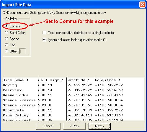
The delimiter selection (comma, tab, semicolon or other) now works. The text qualifier now allows a delimiter in an expression.



Pathloss 5 - revision date February 23, 2010

Create PTP/PTMP links - Design links - Edit modify links

The windows hierarchy in these functions could result in the current window being hidden.



Terrain data section

The survey angles function returns an error message if the cursor is on site 1 - the first point in the profile.



The single structure dialog warning message "Structure exists at this location" has been removed from the dialog. An error message will be generated if the user attempts to add a structure at a location where one already exists.



Multipath - Reflections

Under certain non line of sight conditions, the program would crash when the define plane function was called.



GIS configuration - Indexing NED bil files

This can now be carried out for complete folders and sub folders. In the File index display, click Files - Import index - bil, hdr, blw folder- subfolder. Select the top folder containing these files to create the index.



Pathloss 5 - revision date February 8, 2010

Google Earth Export

Local and area studies are now reprojected from the network display projection to the Google Earth plat carree projection. This improves the positioning within Google Earth, especially for large areas.



Local and Area Studies

If the variables "show local study" or "show area study" are changed in the site list, the changes did not take effect until the local or area study was regenerated. In this program build the changes will take effect immediately when the site list is closed.



Interference case detail report

The delete case and delete subcase buttons in the case detail report would cause a crash whenever all subcases associated with a receiver were deleted



Radio Lookup table

The second time the radio lookup table was accessed, the radio data would not be added if the design section had changed between accesses.



Local studies did not export to Google Earth unless all options were selected



Pathloss 5 - revision date January 20, 2010

Diffraction

If the diffraction algorithm was set in the PL50L program options, the tool bar in the the diffraction section was not reset.



Switching diffraction algorithms in the diffraction section, did not completely reset the calculations resulting in some interaction between algorithms.



Fixed bug in ray trace and reference plane analysis which would not show colors when printed in a batch report.



Pathloss 5 - revision date January 13, 2010

Diffraction loss

Reflective plane definition for Longley and Rice algorithm revised for line of sight applications.



Interactions between the diffraction loss calculations carried out in the transmission analysis section and the diffraction section have been eliminated



Pathloss 5 - revision date January 4, 2010

Some stability problems have been corrected in the link text import. If a file could not be saved, an error report is written and displayed at the end of the import.



Reflection plane report crash.



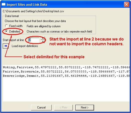
Import text files

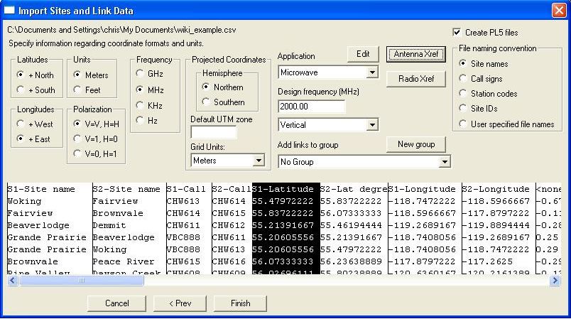
The settings and column definitions can be saved and loaded. This makes it possible to handle any number of column definition formats for a particular import.



Pathloss 5 - revision date December 23, 2009

New menu item Assign Thematics under the Operations menu in PL50 allows thematics (site Type, site Status, link type, link status and los status) to be assigned to a selection or group.



Exporting to Google Earth now allows the local studies to be exported as a single image rather than an image for each base station. This option is shown on the export dialog.



Exporting PL5 to PL4 was missing the traffic code. This has been fixed



Pathloss 5 - revision date December 17, 2009

Fixed bug which caused local studies to have erroneous loss if clutter files could not be found.



Fixed some minor visibility problems regarding local studies.



GIS configuration

If a vector file (MapInfo or Shapefile) with building elevations was entered in the vector tab file list, then the program would crash when the file list was opened and the vector file was not at the specified location.



Grid ASCII conversion

Improved error detection in grid ascii file



3D terrain view

The user interface has been redesigned.



Update pl5 files

This function in the site data list will set the profile end point elevations to the values specified in the site list.



Automatic OHLOSS calculations in an interference calculation

If the "Calculate OHLOSS automatically" option was checked in an interference calculation, the program calculated the OHLOSS for each case. If the addition of the OHLOSS resulted in an interfering signal less than the objective minus the margin, the interference case was discarded. In all other cases the reports showed the OHLOSS being included twice.



Radio and antenna lookup tables

For antenna, the model and gain are the minimum requirements For radio lookup tables, the model transmit power and receive sensitivity are the minimum requirements. Minor reformatting changes were carried out to these tables.



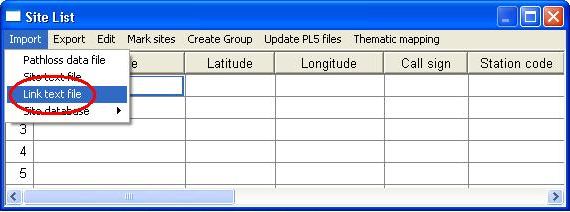
Import link text file

A csv file with more than 2048 characters per line would cause a program crash. Any line length can now be used.



Pathloss 5 - revision date December 02, 2009

Visibility of ungrouped sites and links is saved in the gr5 file.



Export to shapefile and mapinfo mid/mif now allows export of groups or selections. More information exported to shapefile and mapinfo mid/mif databases.



3D Display now only shows visible network.



Fixed error exporting studies to google earth from certain datums.



Refinements to google earth export: More information in description, links now shown above ground at antenna height.



Pathloss 5 - revision date November 25, 2009

Export to google earth now allows export of groups or selection.



Maximum receive signal exceeded has been added to the trasmission analysis warnings.



More information is exported to mapinfo mid/mif format.



Pathloss 5 - revision date November 17, 2009

Profile displays now show the arrow on top of any structure or clutter at the selected point.



The excess clearance display in the antenna heights design section showed the longitude hemisphere incorrectly.



Erroneous base station circulator branching loss values could be generated if the Cancel (red X) button was clicked in the antenna coupling unit data entry form.



Create P2P links. Joining a group (or selection) to all sites now works as it should. Previously, some links between group members were omitted.









Pathloss 5 - revision date November 10, 2009

Create P2P links

Joining a group (or selection) to all sites now works as it should. Previously, some links between group members were ommited.



Hot keys have been added to switch between the link design sections.



Manual site linking direction Manual links were created in west to east direction. Links which were exactly north - south were created in a south to north direction. Using this convention, all profile displays had the westerly site on the left side.



This has been changed so that the first site selected is always on left side of profile displays.



Link text file import If the design frequency is not available in the import, the average channel assignments are now used.



Print profile options

The print profile options were not saved on exiting the report printing dialog.



Pathloss 5 - revision date October 20, 2009

Fixed crash involving Ohloss and Diffraction Loss Reports.



Pathloss 5 - revision date October 15, 2009

GIS Configuration

ESRI header files used for indexing BIL files with out a corresponding prj file are now supported. The projection information is contained in the hdr file. The user must set the projection.



CSV Import

The duplicate column assignments error message now identifies the specific column numbers and in the case of the "Site text file" import, the field name is specified.



The link text import loads the antenna code if available.



Pathloss 5 - revision date October 5, 2009

Rain data files

City rain data files have been added to the program. These are non proprietary rain files for US and Canadian cities.



Provision has been made to use the Proprietary ATT radio data files; however these are not supplied with the program. These files must be located in the directory geo_data\rain\alu_rain.



Radio and Antenna Code Index

Improved functionality for the find control.









Pathloss 5 - revision date September 29, 2009

Link Text Import

Coordinates using separate columns for degrees, minutes and seconds were not importing correctly.



Station, owner and operator codes

These site specific parameters can be used for alternate data storage and status information. These parameters can be excluded from the network



pl5 file discrepancy checking. Click Configure - PL50 Program options

Network link data checks to set these options.

Link design rules

Field margin has been added to the link design rules. The data entry is in the reliability parameters section of the design rules dialog.



Radio and antenna code data entry.

These can now be entered directly and deleted in the respective data entry forms.



Tooltips have been added to the radio and antenna indexes.



Antenna clearance report

If the controlling clearance criteria included a fixed height, the clearance report did not included this fixed height.



GIS Configuration

If the vector tab included shapefile definitions, and the shapefiles were not present, the program could crash on startup.



Pathloss 5 - revision date September 24, 2009

Backdrops

The Import Index - Mapinfo tab file option now supports bmp, jpg, and png in addition to tif as image formats. One bit black and white tif files are now supported.



Link text file import

Multiple links between the same two sites can now be carried out in the link text file import



Pathloss 5 - revision date September 22, 2009

Vertical Mapper Clutter files (gcd files)

Clutter data in the MapInfo vertical mapper format may include a clutter definition table in the file. If this exists the data will be automatically entered into the clutter definition table.



Note that clutter elevations do not exist in this file format. All clutter elevations have been set to a default value of zero. It is the users responsibility to assign the clutter heights. The clutter cross reference categories have been set to an "open land" default value. For local and area studies, the user must assign the cross references



GIS Configuration

The Philippine reference system 1992 datum has been added. This is effectively the same definition as the existing Luzon datum, however the transformation to WGS84 utilizes the 7 parameter algorithm for the entire country, whereas the the Luzon definition uses a 3 parameter transformation and two regions (Philippines excluding Mindanao and Mindanao) The Philippine transverse mercator projection for the five zones has been added for this datum



The clutter definition table now shows the clutter elevations in the units currently selected (feet or meters). Previously units were always in meters



Interference case detail report

Headers in the performance degradation did not line up with the actual data.



PL50L Options

The automatic diffraction algorithm selection (Pathloss, Tirem or NSMA) was not included in the PL50L option settings



Obstruction Fading (transmission analysis section) The diffraction loss iterations could fail under certain conditions and return a critical value of K of 1.33. The results were completely unrealistic



Pathloss 5 - revision date September 15, 2009

Passive repeaters

Passive repeaters created in the network display had stability problems.



Vectors

Added support for displaying ESRI shapefiles of type SHPT_ARCZ and SHPT_POLYGONZ.



Backdrop Files

MapInfo tab files can be loaded directly in to the Backdrop index. This is a multiselect operation. If the list is empty, then the first file added sets the projection. All successive files must match this projection. If the index contains any entries, then the existing projection determines if the file can be accepted.



Update PL5 file in the network display only updated one site in a link if the YES button was clicked. The Yes to all button operated correctly.



GRIDASCII

Converting a GRIDASCII resulted in a "File format error" on UNIX files. The program incorrectly interpreted the 0xA end of line character.



Pathloss 5 - revision date September 8, 2009

Set GIS configuration The MapInfo derived projection could cause a program crash if it was manually selected from the projection drop down list.



The ERP values in watts and dBm were reversed in land mobile applications in the transmission analysis display.



Diffraction loss

The diffraction loss calculation failed on line of sight paths with more than 6 terrain incursions into the 60% Fresnel zone radius.



Pathloss 5 - revision date September 2, 2009

Vertical mapper grd DEM files using 16 bit integers were not correctly read.



Pathloss 5 - revision date September 1, 2009

Link text file import

If the design frequency is not specified, and channel frequency assignments are in the file, then the design frequency will be set to the average of the channel frequencies.



Define plane

The define plane caused a crash when switching between the manual and automatic generation methods



The network file consisted of two files with the suffixes gr5 and gr5ids. The gr5ids contains the site and link ids and is intended to be used on a shared file basis. The gr5ids file has been removed in this program build due to potential data synchronization problems.



Rain errors were reported even when the rain calculation was switched off.



The free space loss formula gave results which were 0.02 dB different than the version 4.0 results. This small difference created difficulties in comparing availability results which are formatted to five decimal places. This release changes the free space loss to the version 4 formula.



Pathloss 5 - revision date August 26, 2009

Minor fixes to radio and antenna lookup tables.



Pathloss 5 - revision date August 25, 2009

Pl50 Options

Site Attributes, Site Label, Link Attributes and Link Labels can now be applied to a group or selection.



Set GIS Configuration

The File index for NLCD2001 clutter did not show the clutter name on the caption



PL40 radome loss

When a pl4 file containing a valid antenna code was opened in the standalone PL50L application, the antenna data was reloaded. This caused the radome loss to reset.



Space diversity - IF combining - corrected.



Changed gr5 save routine to guard against header errors.



Pathloss 5 - revision date August 17, 2009

Transmission summary report when invoked from the transmission analysis menu bar always showed the distance and elevation in Miles / feet



Network to PL5 discrepancy dialog. Direction arrow buttons did not function.



Pathloss 5 - revision date August 13, 2009

Network display - Map crossings

The map crossing function has been implemented. This is only valid for the default network projection. First set the axis to correspond to the desired maps (Click configure - PL50 options - axis-map grid). Then right click on the link and select map crossings. If the US 1:24,000 7.5 minute map scale has been selected, the report will show the actual map names.



Terrain data module

The reverse profile did not reverse the site names on the status bar.



Fixed google earth datum transformation.



Fixed minor bugs related to the no data entries in clutter databases.



Pathloss 5 - revision date August 6, 2009

Group manager

The visibility display rules have been changed to allow a group containing only links to be displayed. Some fixes have been made involving operations where some sites and links are hidden.



Antenna heights section

The graphical antenna heights display now does not show the minimum clearance criteria. Previously this was show as a modification to the Fresnel zone radius. Although the results were correct, this display was somewhat confusing.



The minimum clearance criteria is intended to provide clearance for close in obstructions where K and the Fresnel zone radius are very small and can lead to a grazing path. Note that when this is specified, the antenna heights cannot be less than this value.



Radio data entry form (Adaptive modulation)

Clicking the blue button to access the adaptive modulation table, could bring up a second instance of the table which could cause a program crash.



Update PL5 files has been added. This function is available on the site list menu bar. The procedure checks all associated pl5 files and compares the site data to the data in the site list. If there are any differences the user is prompted to modify the pl5 file. This is a one direction change - Network site data to pl5 file.



Pathloss 5 - revision date July 31, 2009

NLCD2001 and NCLD2002 clutter data downloads in BIL format from the USGS site are now working. These files can be used with the July 31, 2009 program build.



NED and SRTM elevation data downloads in BIL format are now in a 32 bit floating point format. We believe that this is an error as the definition of the BIL format on the USGS site states that the elevations are in a signed 16 bit integer format. The new float files are twice the size of the integer files.



The July 31, 2009 program build will read the floating point files.



The Group manager operation has been revised so that links can exist in a group without the associated sites being in the group. This allows the user to create a group with links only or with sites only. Combinations of sites and links in a group are still possible. In this arrangement, links can now be hidden without hiding the sites.



Printing and copying the network display with backdrops produced black ares where the backdrop was missing.



Pathloss 5 - revision date July 29, 2009

Site list does not reset display unless coordinates are changed.



Set GIS Configuration correctly recognizes when the projection of the display has changed.



Pl5 Link Files deleted by Pathloss are now sent to the recycle bin rather than being permanently deleted.



Reports

Fixed bugs causing columns to be out of sync and filenames to not be displayed in some cases.



Antenna Usage is shown next to the antenna model in the transmission detail and transmission summary reports.



Point to point link design

The antenna coupling unit (ACU) data entry form in the base station definition did not match up with the ACU data entry in the Link Design Rules. These are now exactly the same interface



Pathloss 5 - revision date July 24, 2009

The addition of new fields to site data caused a crash in the site data entry forms.



Fixed error in which a group could become corrupted when importing from site text files.



Pathloss 5 - revision date July 22, 2009

Obstruction Fading

A preliminary implementation is available in the transmission analysis design section. Click Operations - Obstruction fading. The next program build will include the documentation and the obstruction fading will be incorporated into the reports



Local and area studies

The receive at base station option cause an error.



CSV link report

The antenna usage field has been added. This will only appear if the antenna model is checked.



Import text links

Quotation marks were not automatically removed.



A preliminary request for frequency coordination CSV report has been added. Click Operations - Frequency Coordination report. The report format may change based on discussions with Alcatel and Comsearch. The following fields have been added to the site data structure for this report.



Antenna registration number char[16]

Zip code char[16]

Tower height with Appurtenances

Under some circumstances - distance, azimuth and projected coordinates were not automatically calculated from the site coordinates.

SRTM Image Data

Welcome. If you just can't wait to start playing with the SRTM image data, or just don't have the


patience for reading tedious documentation, you'll need to know at least the following. For more detail

see SRTM_Image.doc.

All SRTM data are divided into tiles extending over 1° x 1° of latitude and longitude, in “geographic”

projection. For the DEMs, data from every acquisition that crossed a tile were mosaicked and combined,

so there is only one data file for each 1° tile. However for image data every data take that crossed a tile

is included as a separate file (no mosaicking or combining has been done) and some files may contain

only partial data. In addition, because of the SCANSAR technique involved, each SRTM swath was

made up of four slightly overlapping subswaths. Data from each subswath is also included in a separate

file, so every image pixel acquired by SRTM is included in this set.

There are two files for each subswath included in a tile:

.mag - radar image data

.inc – local incidence angle for each sample in the image file

Naming convention:

- As with the DEM files, the first 6 characters of each file name for image data indicate the

geographic coordinates of the center of the lower left (southwest) sample of each file.

- For image files this is followed by 6 numbers that indicate the data take number, consisting of

the orbit number followed by a serial number for that orbit.

- This is followed by a subswath number, which increases outward from the spacecraft nadir point,

and is the key to the polarization for that subswath.

o SS1 = subswath 1, HH polarization approx 30° - 43° look angle.

o SS2 = subswath 2, VV polarization approx 44° - 52° look angle.

o SS3 = subswath 3, VV polarization approx 47° - 60° look angle.

o SS4 = subswath 4, HH polarization approx 52° - 62° look angle.

- Example: File N07W081_032_010_SS3_1_01.mag has its lower left sample centered on 7°N

latitude, 81°W longitude, was the 10th data take on orbit 32, and includes data from subswath 3

indicating VV polarization.

Format:

- Both image and incidence angle files are sampled at 1 arc second of latitude and longitude (~ 30

meters at the equator), and are in geographic projection (AKA Plate Caree). Thus both files have

3601 samples and 3601 lines. Incidence angle files were first averaged to 3 arc seconds before

sampling to 1 arc second.

- Image files are 8 bits/sample, with the values indicating radar cross section, or brightness, scaled

linearly between -50 dB and +40 dB. Data numbers (DN) can be converted to backscatter cross

section in dB using the expression dB = 0.3529*DN - 50

- Incidence angle files are 16 bits/sample, measured in hundredths of a degree (i.e. 4321 = 43.21°).

The 2 bytes are in Motorola "big-endian" order with the most significant byte first, directly

readable by systems such as Sun SPARC, Silicon Graphics and Macintosh. DEC Alpha and most

PCs use Intel ("little-endian") order so byte-swapping may be necessary

SRTM Images

The SRTM data sets result from a collaborative effort by the National Aeronautics and Space

Administration (NASA) and the National Geospatial-Intelligence Agency (NGA - previously known as

the National Imagery and Mapping Agency, or NIMA), as well as the participation of the German and

Italian space agencies, to generate a near-global digital elevation model (DEM) of the Earth using radar

interferometry. The SRTM instrument consisted of the Spaceborne Imaging Radar-C (SIR-C) hardware

set modified with a Space Station-derived mast and additional antennae to form an interferometer with a

60 meter baseline. A description of the SRTM mission can be found in Farr and Kobrick (2007).

Synthetic aperture radars are side-looking instruments and acquire data along continuous swaths. The

SRTM swaths extended from about 30° off-nadir to about 62° off-nadir from an altitude of 233 km, and

thus were about 225 km wide. During the data flight the instrument was operated at all times the orbiter

was over land and about 1000 individual swaths were acquired over the ten days of mapping operations.

Length of the acquired swaths range from a few hundred to several thousand km. Each individual data

acquisition is referred to as a "data take."

SRTM was the primary (and pretty much only) payload on the STS-99 mission of the Space Shuttle

Endeavour, which launched February 11, 2000 and flew for 11 days. Following several hours for

instrument deployment, activation and checkout, systematic interferometric data were collected for

222.4 consecutive hours. The instrument operated almost flawlessly and imaged 99.96% of the targeted

landmass at least one time, 94.59% at least twice and about 50% at least three or more times. The goal

was to image each terrain segment at least twice from different angles (on ascending, or northeast-going,

and descending, or southeast-going, orbit passes) to fill in areas shadowed from the radar beam by

terrain.

This 'targeted landmass' consisted of all land between 56° south and 60° north latitude, which includes

almost exactly 80% of Earth’s total landmass.

2.0 Data Set Characteristics

All SRTM data are divided into tiles extending over 1° x 1° of latitude and longitude, in “geographic”

projection. For the DEMs, data from every acquisition that crossed a tile were mosaicked and combined,

so there is only one data file for each 1° tile. However for image data every data take that crossed a tile

is included as a separate file (no mosaicking or combining has been done) and some files may contain

only partial data. In addition, because of the SCANSAR technique involved, each SRTM swath was

made up of four slightly overlapping subswaths. Data from each subswath is also included as a separate

file, so every image pixel acquired by SRTM is included in this set. Sample spacing for individual data

points is 1 arcsecond; one arc-second at the equator corresponds to roughly 30 meters in horizontal

extent

There are two files for each subswath included in a tile:

.mag - radar image data

.inc – local incidence angle for each sample in the image file

2.1 SRTM Image Data

The long wavelength of radar waves makes them most sensitive to surface roughness at scales near the

radar wavelength (for SRTM, about 5.5 cm). Thus, for example, rough rocky surfaces, wind-roughened

water, and vegetation appear bright while smooth sand and water appear dark in these images. Of

secondary importance is variations in dielectric constant, which is similar for most dry geologic

materials. However, as water has a very high dielectric constant, wet soils tend to show up much

brighter than dry soils. Several texts are available which describe in much more detail processing and

interpretation of radar images (e.g. Elachi, 1988; Henderson and Lewis, 1998; Campbell, 2002).

As radar images are acquired in a side-looking geometry, they can be distorted by topographic

variations. Because SRTM acquired topography at the same time as the image data and the two are

inherently registered, it was an easy matter to orthorectify the image data. This also means that voids

present in the SRTM DEM produce voids in the image data.

The SRTM radar image product provides the mean surface backscatter coefficients of the mapped areas.

This required the image processor to be radiometrically calibrated. For SRTM, the goals for absolute

and relative radiometric calibration were 3 dB and 1 dB respectively. The SRTM main antenna was the

major source of calibration error as it was a large active array antenna. In the spaceborne environment,

both zero gravity unloading and the large variation in temperature caused distortions in the phased array.

Hundreds of phase shifters and transmit / receive modules populated the C-band antenna panels.

Monitoring the performance of each module was very difficult, causing inaccuracies in the antenna

pattern predictions, in particular in elevation, as the beams were spoiled to obtain a wide swath.

Therefore antenna elevation pattern correction coefficients were derived with empirical methods using

data takes over the Amazon rain forest. As the Amazon rainforest is an homogeneous and isotropic area,

the backscatter coefficient is almost independent of the look angle. Without compensation, a scalloping

effect would have been visible in the sub-swath and full-swath images.

Speckle noise is present in the image data. This is a characteristic of coherent imaging systems and

appears as a random, high-frequency, salt and pepper effect. Most imaging radar systems average many

‘looks’, however SRTM was optimized for a wide swath and thus acquired only 1-2 looks per sub-swath

causing a relatively high speckle noise level.

2.2 SRTM Incidence Angle Data

Because local incidence angle is so important for interpretation of radar images, a file containing that

information is provided for each of the image files. The values are calculated from the position of the

Shuttle and the DEM. They represent the angle between the radar beam and the local normal to the

surface at each pixel. Because this information could be used to ‘back-calculate’ a DEM, the incidence

angle pixels were averaged 3x3 and sampled back to 1 arc-second in order to remain registered with the

corresponding image file.

The figure below shows a portion of cell N34W119, demonstrating the characteristics of the image and

incidence angle data sets and the difference with the topographic data.

Figure 1. Comparison of SRTM image data and SRTM DEM for cell N34W119 (Los Angeles, CA).


Left: Descending sub-swath N34W119_072_100_SS2_1_01. Upper left: Image file, Lower left: Incidence angle file.

Center: Ascending sub-swath N34W119_114_030_SS4_1_01. Upper center: Image file, Lower center: Incidence angle file.

Right: SRTM DEM for the same cell, shaded-relief and elevation color-coded.

Note that the voids in the DEM (shown in grey) correspond to black areas in the image and incidence angle file. The

incidence angle files look like shaded-relief topography because they’re calculated in a similar way. Note that the rough,

vegetated mountains are bright in the images while the smoother Mojave Desert tends to be dark.

3.0 Data Formats

As with the DEM files, the first 6 characters of each file name for image data indicate the geographic

coordinates of the center of the lower left (southwest) sample of each file. For image files this is

followed by 6 numbers that indicate the data take number, consisting of the orbit number followed by a

serial number for that orbit. This is followed by a sub-swath number, which increases outward from the

spacecraft nadir point, and is the key to the polarization for that sub-swath.

o SS1 = sub-swath 1, HH polarization approx 30° - 43° look angle.

o SS2 = sub-swath 2, VV polarization approx 44° - 52° look angle.

o SS3 = sub-swath 3, VV polarization approx 47° - 60° look angle.

o SS4 = sub-swath 4, HH polarization approx 52° - 62° look angle.

Example: File N07W081_032_010_SS3_1_01.mag has its lower left sample centered on 7°N latitude,

81°W longitude, was the 10th data take on orbit 32, and includes data from sub-swath 3 indicating VV

polarization.

SRTM image data are sampled at one arc-second of latitude and longitude and each file contains 3601

lines and 3601 samples. The rows at the north and south edges as well as the columns at the east and

west edges of each cell overlap and are identical to the edge rows and columns in the adjacent cell.

This sampling scheme is sometimes called a "geographic projection", but of course it is not actually a

projection in the mapping sense. It does not possess any of the characteristics usually present in true map

projections, for example it is not conformal, so that if it is displayed as an image geographic features

will be distorted. However it is quite easy to handle mathematically, can be easily imported into most

image processing and GIS software packages, and multiple cells can be assembled easily into a larger

mosaic (unlike the pesky UTM projection, for example.)

3.1 Image File (.mag)

Image brightness or magnitude is given as 8 bits/sample, with the values indicating radar cross section,

scaled linearly between -50 dB and +40 dB. Data numbers (DN) can be converted to backscatter cross

section in dB using the expression dB = 0.3529*DN - 50. There are no header or trailer bytes embedded

in the file. The data are stored in row major order (all the data for row 1, followed by all the data for row

2, etc.).

These data also contain occasional voids from a number of causes such as shadowing, phase unwrapping

anomalies, or other radar-specific causes. Voids have the value 0.

3.2 Incidence Angle File (.inc)

Local incidence angle is provided as 16-bit integer data in a simple binary raster. There are no header or

trailer bytes embedded in the file. The data are stored in row major order (all the data for row 1,

followed by all the data for row 2, etc.). The pixel values represent hundredths of a degree (i.e. 4321 =

43.21°).

Byte order is Motorola ("big-endian") standard with the most significant byte first. Because the

incidence angle data are stored in a 2-byte binary format, users must be aware of how the bytes are

addressed on their computers. The incidence angle data are provided in Motorola or IEEE byte order,

which stores the most significant byte first ("big endian"). Systems such as Sun SPARC and Silicon

Graphics workstations and Macintosh computers use the Motorola byte order. The Intel byte order,

which stores the least significant byte first ("little endian"), is used on DEC Alpha systems and most

PCs. Users with systems that address bytes in the Intel byte order may have to "swap bytes" of the

incidence angle data unless their application software performs the conversion during ingest.

These data also contain occasional voids from a number of causes such as shadowing, phase unwrapping

anomalies, or other radar-specific causes. Voids have the value 0.

Pathloss version 5 - Maintenance update - Build date January 4, 2011

Check the build date of your current installation. Click the Help - About Pathloss 5.0 menu item.

If the build date is May 7, 2009 or newer, then use the link below to download the January 4, 2011 maintenance update.

Pathloss 5 update
This is an InstallShield installation program. The Pathloss program must be closed to run this update

If the build date of the current installation is earlier than May 7, 2009 then the update must be carried out as a new installation as described below.

Pathloss version 5 - Maintenance update using a new installation

Your existing installation must be first be uninitialized and then the program must be removed.

The following steps detail the procedure.

Start the Pathloss program

Click Configure - Pathloss program - Uninitialize program

If you were able to initialize the program on line, then select this option and click the Uninitialize Program button. You will be prompted to proceed with the uninitialization. This step will automatically update the licensing database for the next installation.

If you were not able to initialize the program on line due to the program internet access restrictions, then select the EMail option and click the Uninitialize Program button.

You will first be prompted to proceed with the uninitialization. Once the program has been uninitialized, the dialog on the left will appear. Click the "Copy serial number and uninitialization code" button. This step copies these two item to the clip board.

Create a new Email to cte@pathloss.com and paste (Ctrl V) the serial number and uninstallation code into the EMail body.

When we receive the EMail, the licensing database will be updated for the next installation.

Note that the uninitialization procedure (on line and EMail) creates the file "pluninst.txt" in the tmp_file folder. This file contains the serial number and uninstallation code. This also can be Emailed to update the installation status

Once the program has been uninitialized, remove the Pathloss program using the Control Panel operation "Add or Remove Programs" to remove the Pathloss program.

Finally download and install the latest program build using the procedure supplied with your serial number notification

Important note to VISTA users
It will be necessary to manually delete all files in the directory

C:\Users\\AppData\Local\VirtualStore\Program Files\Pathloss 5\geo_data

before installing the complete program.